
Lesson 17 – The Land Residual Techniques of Income Capitalization (The Income Approach to Value)
The material in this lesson will be very familiar with what was studied in Lesson 16; the residual techniques are similar. (1) First determine the income the property will earn under the highest and best use. (2) Using "IRV", determine the income imputable to the known value component. (3) Subtracting the income attributable to the known value component from the total property income leaves you with the income residual to the unknown value component. (4) Use "IRV" to capitalize the income residual to the unknown value component into value.
As was mentioned in Lesson 15, the appropriate capitalization rate for improvements must make an allowance for recapture (return OF the investment), as well as for yield (return ON the investment) and ad valorem property taxes. In this Lesson we will make an allowance, in determining the income imputable to the improvement(s), for the investment in the wasting asset.
The previous lesson, Lesson 16, discussed the:
- Building Residual Technique
- Straight-Line Declining Terminal Income to the Building
- Level Terminal Income to the Building
This lesson discusses the:
- Land Residual Technique
- Straight-Line Declining Terminal Income to the Land
- Level Terminal Income to the Land
What is a "Residual Technique"?
We will discuss the land residual technique in this Lesson; the building (improvement) technique was discussed in the previous lesson, Lesson 16. The building residual technique is used when the land value is known; the land residual technique is used when income to an improvement can be obtained. Both techniques are basically the same – starting with the total income imputable to the property, the income imputable to one of the components (improvements or land) is deducted, which leaves the income residual to the other component, which is then capitalized into value, using the appropriate valuation method and rate.
Property Tax Rule 8, previously covered in Lesson 5, "Definition of the Income Approach and Property Tax Rule 8", states, regarding the income approach to value:
… It is the preferred approach for the appraisal of land when reliable sales data for comparable properties are not available. …
In subsection (b) this topic is expanded:
(b) Using the income approach, an appraiser values an income property by computing the present worth of a future income stream. … In practical application, the stream is usually either
…
(2) divided horizontally by projecting a perpetual income for land and an income for the economic life of the improvements, …
…
It is the horizontally divided income streams that we discussed in the previous lesson and will primarily discuss in this Lesson; in Lesson 18 we will learn about the income streams described in subsection (b)(1).
Residual techniques allow for capitalization of an income stream allocated to an investment component of unknown value once all investment components of known value have been satisfied. An appropriate capitalization rate is applied to the value of the known components(s) to derive the annual income needed to support the investment in that component. The annual income of the known component(s) is deducted from the net income before recapture and taxes to derive the residual income available to the unknown component. The residual income is capitalized using an appropriate capitalization rate to derive the present value of the unknown component. The final step is to add the value(s) of the known components(s) and the value of the residual component to derive a value indication for the total property.
In Lesson 15 we learned that the appropriate capitalization rate for land – which is theoretically assumed to exhibit a constant perpetual income stream, is a combination of a yield rate (Yo) and an effective tax rate (ETR). As was mentioned in that Lesson, the appropriate capitalization rate for improvements must make an allowance for recapture (return OF the investment), as well as for yield (return ON the investment) and property taxes.
How an allowance for recapture is determined depends on the shape of the income stream. If the income stream is forecast to be straight-line declining terminal, the rate for the recapture allowance is the reciprocal of the Remaining Economic Life [REL] – that is, it is calculated by dividing the number one (1) by the REL; the rate of recapture is also known as the Capital Recovery Rate [CRR]. If the income stream is forecast to be constant (level) terminal, the CRR is the sinking fund rate, based on Yo, for the wasting asset’s REL.
Let’s rephrase these previous paragraphs. The residual techniques we are discussing will be used for the valuation of improved properties – either actually improved, or with proposed improvements. Using a residual technique, (1) the appraiser needs to know what the property will earn, either as improved, or as it might be improved. (2) The appraiser needs to know the information necessary to develop the capitalization rates – yield rate, capital recovery rate, and effective tax rate. And (3) the appraiser needs to know the value of one of the components of the improved, or hypothetically improved, property – either a building value or a land value.
- First determine the income the property will earn under the highest and best use.
- Using "IRV", determine the income imputable to the known value component:
- If you know the land value, then the land income is the land value times the land capitalization rate; IL = RL × LV, where the RL = (Y + ETR).
- If you know the building value, then the building income is the building value times the building capitalization rate; IB = RB × BV, where the RB = (Y + CRR + ETR).
- Subtracting the income attributable to the known value component from the total property income leaves you with the income residual to the unknown value component.
- Use "IRV" to capitalize the income residual to the unknown value component into value.
- If you knew the land value, then your residual income is the income to the building; BV = IB ÷ RB, where the RB = (Y + CRR + ETR).
- If you knew the building value, then your residual income is the income to the land; LV = IL ÷ RL, where the RL = (Y + ETR).
- Adding the known component value to the value just derived will result in the total value.
Reviewing the Concepts that are the Basis of the Residual Techniques
Lesson 6, Characteristics of the Income Stream, discussed the shapes of five different income streams: (1) Constant Perpetual; (2) Level (or Constant) Terminal; (3) Straight-Line Declining Terminal; (4) Variable Income; and (5) Single Income Payment (Reversion). In this lesson we will apply appraisal models to the first three of primary income patterns. In the next lesson we will continue using the Constant Perpetual and the Level Terminal streams, and also examine the last pattern, the Single Reversion Payment; in Lesson 19 we will conclude this area of discussion when we apply the Level Terminal annuity and the Reversion payment in the appraisal of leased personal property.
Lesson 8, Capitalization, discussed "IRV", Income = Rate × Value, and also discussed the use of Factors and Multipliers, comparing them to Rates. We said that, from a purely theoretical point of view, a Rate could be thought of as the reciprocal of a Multiplier or Factor.
Lesson 10, Rates and Factors, further discussed the relationship between rates and factors.
Hereinafter, when we use the term, "Rate", such as in “IRV", I = R × V, "Income equals Rate times Value”, we may be using it as a multiplier, quotient, divisor (or denominator), or as the result of a calculation — a quotient or product.
- In I = R × V, a multiplication calculation, R and V are the multipliers, and I is the product.
- In R = I ÷ V, and R = Ant I ÷ SP, division calculations, R is the quotient, I is the dividend (or numerator), and V (or SP) is the divisor.
- In V = I ÷ R, another division calculation, V is the quotient, I is still the dividend, and R is now the divisor.
Moreover, when we use the term, "factor", we will usually be referring to a number taken from a compound interest table. Sometimes a factor may be the addend, sum, minuend, subtrahend, or difference in an equation.
- In “SFF + i = PR”, the Sinking Fund Factor [SFF] and the interest rate [i] are the addends and the Periodic Repayment factor [PR] is the sum, the result of the calculation.
- In “PR − i = SFF”, PR is the minuend, i the subtrahend, and SFF is the difference, the result.
As bulleted in the previous section, we will discuss two residual techniques in this Lesson, the building (improvement) technique and the land residual technique. Both techniques are basically the same – starting with the total income imputable to the property, the income imputable to one of the components (land or improvements) is deducted, which leaves the income residual to the other component, which is then capitalized into value.
Land Residual Technique
As stated in Lesson 15, “Land Valuation”, the most reliable method of estimating land value is through the comparison of the subject property with recent sales of comparable, similarly located, properties. Since the value of all land is based on its productivity, or income producing ability, when utilized at its highest and best use, it is also appropriate to use the income approach to value; this is especially true whenever the comparative sales approach is inapplicable, either because of the absence of market transactions or because of the nonexistence of comparable unimproved land, the appraiser may need to turn to the income approach.
The land residual technique is used when the value of the improvements is known, or can be estimated, but the value of the land is unknown. After processing the market income stream of the subject property to the Net Income Before making any deductions for recapture and property Taxes level [NIBT], the income imputed to the improvements is deducted. The residual income is attributable to the land and may be converted to an estimate of land value using a land capitalization rate.
Land Residual Technique – Straight-Line Declining Income Stream
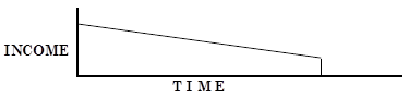
See the shape of a straight-line declining terminal income below; it illustrates a series of annual incomes that decline in equal amounts over a period until the income of the wasting asset terminates. This premise assumes the net income declines by an equal amount each period, and as a result, the value declines an equal amount each period.
Information needed:
- Type of income stream, that is, straight-line declining terminal or level terminal
- Net Income Before deducting for recapture and property Taxes [NIBT], or the requisite information to derive NIBT
- Building Value [BV]
- Yield rate [Y]
- Effective Tax Rate [ETR]
- Remaining Economic Life of the improvement [REL]
After processing the market income stream to the Net Income Before deducting for recapture and property Taxes level [NIBT], the income imputed to the improvement is deducted (Improvement Income). Improvement (Building) Income is derived by multiplying the Improvement (Building) Value by the factor created by the sum of the Yo plus the ETR plus the CRR. CRR can be derived by dividing the number one by REL. The residual income is attributable to the land (Land Income). Dividing the Land Income by the capitalization rate, which is comprised of the Yo plus the ETR, will give us the Land Value. Adding the Improvement Value to the Land Value will give us the Total Property Value.
This can also be expressed in the following formula:
Where:
EXAMPLE 17–1: Land Residual Technique – Straight-Line Declining Terminal Income Stream
Using the same facts as given in EXAMPLE 16–1 in Lesson 16, except assume a vacant parcel. You don’t know the Land Value, but know that it would cost about $40,000 per unit to build a new 20 unit apartment complex that would be comparable to similar, recently completed, properties in this neighborhood; the new buildings would have a 40 year REL. What is the Land Value?
Land Residual Technique –Level Terminal Income Stream
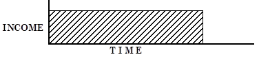
When the income stream is a series of equal, annual incomes that terminate at some point in the future, the income stream is constant terminal shaped.
Information needed:
- Type of income stream, that is, straight-line declining terminal or level terminal
- Net Income Before deducting for recapture and property Taxes [NIBT], or the requisite information to derive NIBT
- Building Value [BV]
- Yield rate [Y]
- Effective Tax Rate [ETR]
- Remaining Economic Life of the improvement [REL]
After processing the market income stream to the Net Income Before deducting for recapture and property Taxes level [NIBT], the Net Income (Before deducting for recapture and Taxes) imputable to the improvement or building (Building Income ≡ NIBTB) is deducted from the total property NIBT. This improvement income [NIBTB] is calculated by multiplying the Improvement Value by the applicable building capitalization rate (YO + SFF{@Yo,Ann,REL} + ETR). The residual income is attributable to the land (Land Income). Dividing the Land Income by the land [NIBTL] capitalization rate, which is comprised of the Yo plus the ETR, will give us the Land Value. Adding the Improvement Value to the Land Value will give us the Total Property Value.
Where:
To arrive at an improvement income, the improvement value is multiplied by the Building Capitalization Rate, RB, which is composed of (1) the Yield Rate YO, (2) the Sinking Fund Factor SFF{Yo, Ann, REL} – the third column in the AH 505, and (3) the ETR. Capital recovery is provided for by including the Sinking Fund Factor in the Building Capitalization Rate.
EXAMPLE 17–2: Land Residual Technique – Level Terminal Income Stream
Using the same facts as given in EXAMPLE 17–1 above, except assuming a level terminal income stream, the Land Value is calculated as follows:
Using the Land Residual Technique to Determine Highest and Best Use
Appraisers sometimes use the land residual technique to determine the highest and best use for the land. Highest and best use is defined as that reasonably probable and legal use that is physically possible, appropriately supported, and financially feasible and results in the highest value. An improvement that is new, and is a probable and legal use, is hypothesized as a starting point. (A new building is hypothesized to eliminate the need to calculate physical deterioration when estimating the value of the building. A proper use is necessary because only under these conditions can the assumption be made that the replacement cost of the new hypothetical improvement equals value – that is, there will not be any deterioration or obsolescence. Several land residuals (different types of land uses) may have to be computed in order to determine which land use returns the highest land value.
This hypothetical improvement value is used only for estimating a residual income to the land. Once this is accomplished, the appraiser does not need to use the hypothetical improvement. The income imputed to the land is capitalized into an indicated land value. The indicated land value, together with other actual information on the property as it exists of the date of value, can be used in the cost or income approach to appraise the existing property.
EXAMPLE 17–3: Land Residual Technique used to Determine Highest and Best Use
You are asked to appraise a vacant square corner lot, 100 feet by 100 feet. The zoning regulations allow three possible uses of the lot:
- a chain drive-through fast food restaurant;
- a one-story office building covering 50 percent of the lot; and,
- a two-story apartment house covering 75 percent of the lot.
Proposal 1 – Drive-Through Fast Food Restaurant
Current ground rents for fast food sites are 25 cents per square foot of ground area per month. Lessee pays all expenses except the property taxes. It would cost $125,000 to build the restaurant and all appurtenant improvements. This 3,000 sq. ft. building would have a 10 year economic life, and the shape of the income-stream, on a typical 10 year lease to a major fast-food chain, would be level terminal. A four percent yield rate would be appropriate for this property.
Proposal 2 – Office Building
The cost of an office building suitable for his neighborhood is 60 dollars per sq. ft; this cost includes all appurtenant improvements, such as the parking lot. An economic monthly income is two dollars per square foot of gross building area. A five percent vacancy allowance appears reasonable. Normal operating expenses (excluding taxes) are estimated to be 25 percent of the effective gross income. This building would have a 50 year economic life, and the shape of the income stream would be level terminal. A 5½ percent yield rate would be appropriate for this type of property.
Proposal 3 – Apartment House
The cost of a two-story, 10-unit, apartment house appropriate for this neighborhood is 50 dollars per square foot of floor area; the cost includes an amount for appurtenant improvements, such as laundry facilities, covered parking, and a swimming pool. A schedule of economic rents shows gross annual income of $200,000. A ten percent vacancy and collection allowance appears reasonable. Expenses (excluding taxes) are estimated at 30 percent of effective gross income. This building would have a 40 year economic life, and the shape of the income-stream would be straight-line declining terminal. A six percent yield rate would be appropriate for this type of property.
Proposal 1 – Fast-Food Restaurant (Direct Land Capitalization)
Proposal 2 – Office Building (Land Residual Technique; Level Terminal Income Stream)
Proposal 3 – Apartment House (Land Residual Technique; Straight-Line Declining)
Proposal 2 produces the highest land value; therefore, it represents the highest and best use of the subject site. The value of the lot, regardless how it is used in the future, is $996,000±.
Notes
Summary
The lesson you just read explained how to use residual techniques to value improved and vacant properties. The next lesson will address valuation the property reversion technique.
Note: Before proceeding on to the next lesson, be sure to complete the exercises for this lesson.